Research Library – Page 14 – Center for Business And Economic Research

Who Pays for Cutting Smog-Causing Emissions?

July 26th, 2019

Who Pays for Cutting Smog-Causing Emissions?

On September 24, 1998 the U.S. Environmental Protection Agency ordered 22 states east of the Mississippi to reduce smog-causing emissions in a move to halt wind-borne air pollution in the Northeast. The order requires states to have a clean-air plan in place by September of this year and controls by 2003. The move is expected to prevent thousands of cases each year of smog-related illnesses such as bronchitis and exacerbated cases of childhood asthma. Nitrogen oxides, referred to collectively as NO_x, are the main smog-causing pollutants. The EPA order requires that by 2003 the 22 states (actually 21 states, since Rhode Island does not have to reduce its emissions) reduce their NO_x emissions by a total of 1.16 million tons annually from 1997 levels. See page 4 for the specific list of states and their required reductions.Large, fossil-fuel burning power plants and automobiles are the major sources of NO_x emissions. The EPA estimates that it will cost $1,500 per ton of NO_x reduction by utilities, compared to $3,400 per ton by automobiles. Thus, the EPA advocates focusing on power plants and estimates that the reduction can be achieved by adding $1 to the average consumer’s bill. Some industry and state environmental officials disagree. They distrust EPA’s estimates regarding wind-borne smog traveling to the Northeast and EPA’s estimate of the pollution-reducing cost per electricity consumer. These concerns raise the question: Who pays for NO_x reduction to benefit only the Northeast? In other words, does the EPA Order burden the states equitably?

Trendline analyses between states’ required NO_x reductions and selected economic and demographic data reveal several interesting facts.

On cursory inspection it would seem that states with larger populations are being required to reduce more; however, the percentage reduction is independent of population size. States with lower per capita income are being required to reduce more, in both amount of and percent reduction, so that the poor are being asked to bear a greater burden. States that use more electricity are required to reduce more emissions, making the EPA Order seem fair. However, states that generate and export electricity have an even higher burden.Although automobile NO_x emission reduction is more costly, some experts advocate placing the burden on the driver who is using the road and causing the smog. But automobiles are not the main focus of the EPA Order. Electricity is being targeted, even though it is not fair to burden every electricity consumer equally, when the benefits are primarily for one section of the country.

What does all this mean for Alabama? Alabama’s low per capita income indicates a lower ability to afford clean air and health benefits for our northeastern sisters, even if we are willing to pay for that. Alabama is also a net exporter of electricity—a factor for which the state should receive credits rather than blame. Thus, the state is being targeted unfairly to bear the cost of benefits to the Northeast.

Alabama has local emissions problems to deal with. The air in some of our own counties is not clean. Adopting emissions controls on vehicles would help alleviate the local pollution. And, we are also required, somehow, to help pay for cleaning the air in the Northeast.

Samuel N. Addy

States Required to Reduce Smop-Causing Emissions

	Nitrogen Oxide Emissions
	to be Cut by the Year 2003
		Percent	Electricity, 1997		Miles of	Federal, Public,
		Reduction from	Use	Generation	and Interstate	Per Capita
STATE	Tons	1997 Levels	(million KWh)	(million KWh)	Road, 1995	Income, 1997

Alabama	59,934	27	73,410	113,684	117,714	$20,599
Connecticut	3,234	7	28,377	13,228	26,569	35,954
Delaware	2,413	12	10,025	6,579	7,110	28,443
Georgia	63,158	26	100,400	101,780	142,671	23,893
Illinois	100,965	32	125,882	131,138	173,627	27,927
Indiana	114,169	36	88,400	110,466	116,053	23,183
Kentucky	75,298	33	75,748	91,558	88,143	20,599
Maryland	21,182	23	56,481	44,553	37,586	28,571
Massachusetts	1,647	2	47,543	33,899	42,013	31,207
Michigan	88,842	30	97,029	89,565	151,991	24,998
Missouri	60,556	35	65,268	71,073	154,148	23,723
New Jersey	9,961	9	66,495	23,761	45,498	32,233
New York	10,590	6	131,602	108,099	139,775	30,299
North Carolina	61,449	29	108,439	107,371	118,159	23,174
Ohio	132,728	36	156,606	141,249	144,019	24,203
Pennsylvania	79,338	24	126,512	177,167	147,396	25,578
Rhode Island	–	–	6,680	3,563	7,547	25,589
South Carolina	29,281	21	67,798	78,374	82,414	20,551
Tennessee	69,950	28	86,001	93,293	103,428	22,752
Virginia	35,331	18	87,242	58,986	91,340	26,172
West Virginia	97,967	51	26,224	88,284	45,920	18,734
Wisconsin	38,851	27	59,943	48,560	139,776	24,199

Sources: U.S. Department of Commerce, Bureau of Economic Analysis; U.S. Department of Energy, Energy Information Administration; U.S.
Department of Transportation, Federal Highway Administration; and Environmental Protection Agency.

Alabama Retail Sales Show Strong Increase in 1998

July 26th, 2019

Alabama Retail Sales Show Strong Increase in 1998

Alabama merchants rang up $37.8 billion in taxable retail sales during 1998, according to the Center for Business and Economic Research at The University of Alabama. The Center compiles its reports using data from the Alabama Department of Revenue. Total 1998 sales were 5.8 percent above the $35.7 billion tallied in 1997. Retail sales across the U.S. rose 5.0 percent in 1998. With inflation for the year at just 1.6 percent, Alabama’s 5.8 percent gain translates to a real increase of 4.2 percent. In contrast, the real gain in total sales in the state in 1997 was only 1.8 percent.

Retail sales growth for the year was strongest in the general merchandise category, where 1998 sales were 10.1 percent above 1997 sales. This outpaced average U.S. gains of 6.6 percent. While Alabama hardware and lumber store sales posted a 7.9 percent gain, growth fell short of the 10.4 percent increase nationwide. The state’s automotive group saw sales climb 7.5 percent for the year, above the average U.S. increase of 5.7 percent.

Across Alabama, apparel sales gained 6.7 percent during 1998 and sales at eating places rose 5.2 percent. Nationally, apparel sales were up a lesser 5.2 percent, while furniture stores saw stronger sales gains averaging 8.6 percent. Although Alabama retail sales increased in all categories, sales growth was slow at food stores, up 2.0 percent, and gas service stations, which posted a 1.0 percent gain.

Automotive purchases claimed the largest share of Alabama’s retail sales in 1998, with 18.9 percent of the total. General merchandise stores captured 15.7 percent of the retail dollar, while food stores took in 15.0 percent during the year. Sales shares by category have shifted during the 1990s. In 1990, food stores claimed the largest share of sales with 18.4 percent, while automotive sales were second at 17.3 percent, and general merchandise stores accounted for 13.7 percent.

From 1990 to 1998, total retail sales in Alabama increased 54.3 percent. Lumber and hardware sales led the way with an 83.1 percent climb. Sales of general merchandise were up 77.2 percent, while furniture sales climbed 74.2 percent. The first eight years of the decade also saw gains of 68.3 percent in automotive sales and 66.7 percent in sales at eating places.

The Center for Business and Economic Research has been compiling data on retail trade in Alabama for almost 70 years. Graphs and tables of retail trade data published in the May 1999 issue of Alabama Business & Economic Indicators may also be accessed.

Carolyn Trent

Alabama Gains Residents from Migration in 1997-98

July 26th, 2019

Alabama Gains Residents from Migration in 1997-98

Alabama continued to gain new residents from interstate and international migration between 1997 and 1998, but at a slower pace than during the previous year. According to IRS data, 96,693 individuals moved into Alabama from other states and foreign countries, while 88,740 moved out. This amounts to a net increase of 7,953, below the 10,423 new residents added during 1996-97.

The largest exchanges of residents were between Alabama and Georgia and Florida. From 1997 to 1998, 15,682 Alabamians moved to Georgia, while 14,181 Georgians moved to Alabama, for a net loss to Alabama of 1,501 residents. In contrast, the exchange of 12,621 Floridians moving in and 12,060 Alabamians moving out to Florida netted the state 561 residents.

Overall, the largest net gains of new Alabamians were from Missouri (2,495), Illinois (1,532), New York (848), Michigan (608), and California (562). While Alabama lost residents to 12 states and the District of Columbia, most of the outflows were about 100 or less. After Georgia, only Tennessee (768) and North Carolina (388) netted many Alabama residents.

While Alabama experienced population growth from migration during 1997-98, the gain of 7,953 reported by the IRS is well below that of many southern states. Florida saw the largest net influx of residents (114,483), followed by Georgia (59,982), North Carolina (54,234), South Carolina (23,775), and Tennessee (21,972). Louisiana saw the loss of 12,642 residents during this period, while Mississippi gained 2,702 and Kentucky netted 6,113.

The Internal Revenue Service also calculates median adjusted gross income (AGI) for in-migrants and out-migrants. Alabama was one of four southern states where the median AGI of those moving in ($19,778) exceeded that of those moving out ($19,564). And, at $22,655, the median AGI of Alabamians who stayed in the state was substantially higher than for those who moved in or out.

Note that these IRS data do not provide a complete count of migrants since they only count taxpayers and their dependents. The Census Bureau uses additional records to arrive at its estimate of total net migration into Alabama from 1997 to 1998 of 11,431. By Census Bureau estimates, Alabama gained 126,168 residents from migration between April 1, 1990 and July 1, 1998. However, no detail of interstate movement is available for these totals.

**05/99

Alabama’s Median Age Climbs between 1990 and 1998

July 26th, 2019

Alabama’s Median Age Climbs between 1990 and 1998

The median age of Alabama’s population rose to 35.5 years in 1998, compared to a median of 32.9 in 1990. This means that equal numbers of Alabamians are older and younger than 35.5. Alabama’s median age was higher than that of the South and the U.S. as a whole—both had medians of 35.2 years.

Alabama’s estimated median age climbed from 32.9 in the 1990 census, an increase of 2.6 years, while the U.S. population aged by 2.4 years. This difference is reflected in the growth of the 65 and over population between 1990 and 1998—while Alabama’s elderly population grew by 10.8 percent during this time, the U.S. saw a 9.4 percent gain. In 1998, 13.1 percent of Alabama’s population was 65 and over, compared to 12.7 percent of the U.S. population.

Median age for the state’s men reached 34.1 years in 1998, right at the U.S. median and just above the median for the South of 34.0 years. With more elderly women than men, the median age for women in Alabama was 36.8 years. This compares to 36.3 years for both the South and the U.S. Median age for Alabama’s men rose more rapidly than the median age for women between 1990 and 1998.

Among the states, West Virginia’s population was the oldest with a median age of 38.6 years, while Utah was the youngest with a median age of 26.7 years. By region, the highest median age in 1998 was in the Northeast (36.6 years), followed by the Midwest (35.4 years), the South (35.2 years), and the West (33.9 years).

How Do Southerners Spend Their Money?

July 26th, 2019

How Do Southerners Spend Their Money?

The three biggest items on which Southerners spend their money are, in order, housing, food, and transportation. This is true for the United States as a whole, but Southerners are paying bigger portions of their incomes on transportation and smaller portions on housing than the national average. The U.S. Department of Labor’s Bureau of Labor Statistics conducts a Consumer Expenditure Survey every year. The results for 1997 were recently released.For this analysis, “Housing” includes what people spend for their dwellings (mortgage or rent), property taxes, and utilities and public services (gas, electricity, water, telephone, etc.), but not housekeeping supplies, household furnishings and equipment, or appliance and furniture repair, pest control, housekeeping services, or lawn care services. Southerners use about 23 percent of their total expenditures for housing; the national average is 25 percent.

We include in “Transportation” the purchase and maintenance of new and used cars, trucks, campers, motorcycles, etc., as well as the gasoline, diesel fuel, and motor oil needed to run those machines. Southerners allocate 13 percent of their total spending for those things, as opposed to 11 percent as a national average. Most of the difference is because Southerners buy lots of cars, trucks, and gasoline to run them. Public transportation is in a different category. Although the average dollars spent for public transportation is higher nationally ($393 per year) than in the South ($243), those amounts represent about 1 percent of spending for both groups.

Nationally, Americans, including Southerners, allocate about 14 percent of their budget for food, not counting alcohol. These expenditures include food at home and in restaurants. How people decide to spend their food dollars, whether in fast food restaurants, traditional restaurants, supermarkets, health food stores, etc. tends to relate more to their age, family situation, and lifestyle than the part of the country they live in. A single person under age 25 anywhere in the country is likely to spend a bigger portion of his income in restaurants than a married couple with small children.

Interestingly, Southerners spend about the same amount of money on clothes ($1,507) as they do on entertainment ($1,561). Southerners spend 5 percent of their budgets for entertainment and another 5 for clothes, jewelry, and shoes. “Entertainment” expenses are things such as fees and admissions, televisions, radios, or sound equipment, and also money spent on pets, toys, and playground equipment.”Health care” includes health insurance, medical services, drugs, and medical supplies. Southerners are spending a little bit more on health care, both in dollars ($1,902) and as a percent (6%) of total spending, than the national average ($1,841 and 5%).

Southerners give 3 percent of their budgets for cash contributions, and 9 percent for insurance and pensions. They spend 2 percent for personal care products, 1 percent for tobacco, 1 percent for alcohol, and 1 percent for education.

The Department of Labor’s expenditure data should be used with care. The amounts are averages. An individual household may spend more or less than the average, depending on its particular characteristics. In any geographic region, income, age of family members, and taste influence expenditures. Nevertheless, the Consumer Expenditure Survey gives us a fascinating view of how the South is similar to, and different from, the rest of the county.

Annette Jones Watters

For more information: Contact the Bureau of Labor Statistics Regional Office in Atlanta at (404) 331-3415 to ask for Report 927, Consumer Expenditures in 1997

Jefferson County Has Most Dynamic Population, UA Data Center Reports

July 26th, 2019

JEFFERSON COUNTY HAS MOST DYNAMIC POPULATION, UA DATA CENTER REPORTS

The population of Jefferson County is the most dynamic of any county in the state. The good news is that Jefferson County is home to three of the top-20 fastest growing cities – Morris, Trussville and much of Hoover. The bad news is that it also is home to five of the nine cities that have lost more than 1,000 people since 1990 – Fairfield, Homewood, Mountain Brook, Bessemer and Birmingham.

The net result is that Jefferson County now has about 8,000 more residents than it had in 1990, despite the loss of an estimated 12,350 residents by Birmingham, the county’s chief city.

The latest figures are U.S. Census Bureau data released by the Alabama State Data Center at The University of Alabama, part of the Culverhouse College of Commerce and Business Administration.

The numbers show that Shelby County, Birmingham’s neighbor to the south, has six of the state’s fastest growing towns: Alabaster, Pelham, Hoover, Harpersville, Vincent and Helena. In fact, in terms of percent of change, Helena led, jumping from 4,303 in 1990 to 9,518 July 1, 1998, an increase of 5,215 residents, or 121.2 per cent change. And the area continues to explode.

“These cities are part of a metropolitan statistical area gaining significantly in population,” said Annette Watters, manager of the Alabama State Data Center and assistant director, Center for Business and Economic Research. “Similar situations can be found in the north, east, south and west sections of the state.”

Of the 42 Alabama cities that posted gains of at least 1000 people over the past ten years, only 10 were not part of a metropolitan statistical area.

“Albertville and Arab are strong-growing cities that do not have metro area status, but they are strategically well-placed,” Watters said. “Albertville added more than 2,000 and Arab added more than 1,000. These growing cities are in Marshall County, which has borders touching the Gadsden, Decatur, Huntsville, and Birmingham MSAs.”

Over the past decade Auburn and Opelika in Lee County have shown strong growth rates. Auburn gained 6,595 people and Opelika gained as many as 2,370 people.

Alabama towns have notably interesting changes and stable population sizes. Since 1990, 60 percent of Alabama’s towns have not changed by more than 100 people.

The 10 largest cities in the state, in order, and the percent of change since 1990 are Birmingham (-4.7), Mobile (+1.1), Montgomery (+3.5), Huntsville (+10.1), Tuscaloosa (+7.1), Hoover (+48.9), Dothan (+5.4), Decatur (+9.6), Gadsden (-.9) and Auburn.

In the state of Alabama there are 444 incorporated towns and cities and the 1998 population estimates each are available on the CBER/ASDC web site at http://cber.cba.ua.edu.

Consumer Spending and Consumer Debt

July 26th, 2019

Consumer Spending and Consumer Debt

The United States’ Gross Domestic Product (GDP), the total value of all goods and services produced in the nation, has four major components:

private consumption,
investments,
net exports, and
government expenditures.

A big change in any of these will alter economic activity and the rate of economic growth. For instance, in 1998, a financial crisis and an economic recession in most of Asia caused economists to lower their forecasts of the nation’s economic growth for the year. The reasoning was that a recession in Asia would reduce demand in Asian markets for U.S. exports.

Although net exports declined (meaning higher trade deficits), American consumer spending increased. The economists’ low forecasts were not entirely accurate. U.S. exporters felt the pinch; U.S. retailers did not.

Private consumption, or the personal expenditures of American consumers, is the largest of the four components of GDP. On average, it accounts for about 68 percent of total GDP annually. Total inflation-adjusted GDP and consumer expenditures in 1998 were $7.5 trillion and $5.2 trillion, respectively (in 1992 dollars). Put this way, in 1998 private consumption was 69.3 percent of GDP. However, the contribution of consumer expenditures to economic growth is actually even more important than these numbers indicate. In 1998 the U.S. economy grew by 3.9 percent. Consumer spending accounted for 85 percent of that growth.

Consumer spending in 1998 was primarily fueled by a low inflation rate, strong job growth, strong housing demand, and to some extent the rise in stock market valuations. Energy, commodity, and import prices have been generally low. The economy’s strong job growth is reflected in the low unemployment rate. Housing demand is at an all-time high, and the stock market continues to exceed expectations.

Consumer spending in 1998 increased by approximately five percent in real terms. Purchases of durable goods have been particularly surprising. Consumers increased their purchases of big-ticket items by more than 12 percent. However, the increase in consumer spending has been accompanied by high consumer debt levels and low savings rates. The savings rate dipped below zero percent and has remained at that level in recent months. Consumer outstanding credit reached $1.3 trillion (approximately 21 percent of total disposable income, or 15 percent of total nominal GDP) in 1998. Total household debt,

which on average has increased by about $300 billion a year since 1990, increased by almost $450 billion in 1998. This increase raised total household debt to approximately $5.9 trillion, about 68 percent of GDP.The spending public does not seem to be worried about having more debt or less savings. Recent estimates of consumer confidence and expectations indicate no significant reversal in consumer spending is expected in the near future, and both indexes hit their historic highs in June of 1999. Despite a spending spree, the inflation rate at both wholesale and retail levels has remained in check, providing an added incentive for consumers to spend.

Implications for Alabama

The high rate of consumer spending has been a significant factor in the state’s job growth during recent months. From 1997 to 1998, most of the job growth in Alabama was in the trade and services sectors. Retail and wholesale trade accounted for approximately 30 percent and services businesses accounted for about 50 percent of the 39,600 net new nonagricultural jobs created. In comparison, of the nation’s 3.1 million new nonagricultural jobs, the trade and services sectors accounted for approximately 19 percent and 48 percent, respectively. We can see that Alabama’s economy relies much more on retail trade for creating new jobs than does the U.S. economy. A sharp downturn in consumer spending would seriously affect the state’s job growth.

According to a recent consumer survey published by the U.S. Department of Labor, average before-tax household income in the South was $35,691 in 1997. The same year, the average household in the South spent $32,226, or 90 percent of its income. One rule of thumb tells us that disposable income usually averages about 84 percent of total income. If in the South that number is 90 percent, it is evident that some Southerners are financing their purchases by sources other than household income. Southerners are spending their savings, or they are borrowing more heavily, to supplement their income.

Although no slowdown in consumer spending is expected in the very near future, today’s spending levels cannot be sustained over the long run. Several things could happen. One scenario is that the Federal Reserve might notch the short-term interest rates higher if there are significant signs of increasing price pressures. An interest rate increase would likely reduce both consumer confidence and retail spending, particularly the part of spending being financed by consumer credit. Slower retail spending would surely retard Alabama’s job growth.

Ahmad Ijaz

Percent Nonagricultural Job Growth in Alabama
from Retail and Wholesale Trade

Percent

ab0899chart.jpg (30446 bytes)
Year

Source: Alabama Department of Industrial Relations and Center for
Business and Economic Research, The University of Alabama.

Employment in Alabama’s Rural Counties and Retail Sales in Alabama’s Metropolitan Areas

July 26th, 2019

Employment in Alabama’s Rural Counties

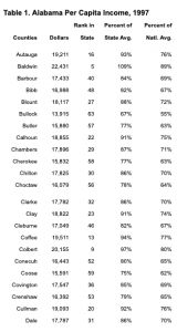
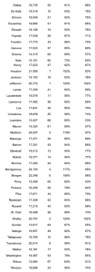
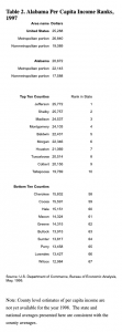
From July 1998 to July of 1999 Alabama’s manufacturing firms lost 9,300 jobs. Sixty percent of the lost manufacturing jobs were in textile and apparel industries. Of the 5,500 jobs lost in these two industries, 4,800 were in rural areas. Most of these jobs were in plants requiring a relatively low-skill labor force and labor-intensive production methods. Because so many jobs are leaving rural counties, economic development there has become an important issue. One difficulty that industry recruiters face is the business world’s relentless change from low- skill, labor-intensive jobs to jobs that require higher educational attainment and technological skills. Many of Alabama’s rural counties have disproportionately high numbers of adults with low levels of formal education or technical training. Thirty-seven of Alabama’s 46 rural counties have an adult population where less than 60 percent have completed a high school education.

Most textile and apparel industry jobs requiring a lower skill level and educational attainment were created in rural areas. Those areas had lower labor costs and provided rural residents with alternatives to employment in the agricultural sector. When an apparel plant has relocated or shut down, displaced workers have had few other employment opportunities. Jobs being created today require higher educational levels and more technological skills than the workforce possesses in some counties.

Employment in textiles and apparel has been declining for quite some time, and NAFTA (North American Free Trade Agreement) probably accelerated the process. One of the choices for workers who have lost their jobs in any industry due to NAFTA has been to apply for Transitional Adjustment Assistance, a Department of Labor program under which workers can qualify for training and assistance. This program has both advantages and disadvantages for the participants. Although the workers attain marketable skills, under most circumstances, the newly-trained people must relocate because the relevant new jobs are in metropolitan areas, rather than the rural areas where they reside. Many former apparel workers cannot relocate. They have obligations that make it difficult for them to move. Since NAFTA’s implementation through the third quarter of 1998, the state has lost 25,000 jobs in the textile and apparel industries. However, only about 3,900 people have applied and been certified for Transitional Adjustment Assistance.

At present there are nine counties in Alabama with unemployment rates over 10 percent and 27 counties with unemployment rates between 5 and 10 percent. Economic development officials desperately want to improve the employment opportunities in those counties. But, there are obstacles. Studies and surveys have shown that manufacturing firms contemplating relocating to rural areas repeatedly mention the same reasons for not doing so. These include lack of:

A skilled labor force
Attractiveness of the area to professional and managerial staff
Accessibility to major cities, markets, airports or other required services
Quality schools and education
Access to suppliers.

Technology and automation are constantly increasing in the industrial sector. Most manufacturing firms do not locate in rural areas because those areas lack a skilled work- force. And the rural workers who become skilled leave the area to take jobs elsewhere. The state’s economic development strategies could use several approaches in order to attract industries to rural counties. Some of these include:

Initially training and retraining rural workers for jobs that require high skills and education
Infrastructure or tax incentives for firms willing to relocate to these rural areas, and
Cooperative programs with private industries to retrain the existing labor force.

Although it is a complicated issue, there are some simple economic realities in this conundrum.

Low-skill jobs will continue to erode.
Industry will locate where it can find a suitable workforce.
There is no short-term quick fix regarding employment issues in Alabama’s rural areas.

The solution lies in long-term investments in education and retraining so high skill, high tech jobs of the future can come to rural areas. Quality schools and other educational programs will attract both professional and managerial staff to these counties. It will take a joint effort of state and local agencies, private firms, and the local citizenry to rescue Alabama’s rural areas.

Ahmad Ijaz

Retail Sales in Alabama’s Metropolitan Areas

Retail sales in Alabama totaled $37.9 billion in 1998, 6.0 percent above the $35.7 billion rung up in 1997. Across the state, 1998 growth was strongest in sales of general merchandise, up 10.1 percent; hardware and lumber, 8.2 percent higher; and the automotive sector, where sales climbed 7.8 percent. At 2.1 percent, food store sales showed the slowest growth. The average Alabamian spent $8,709 on retail purchases in 1998. Sales for the first four months of 1999 were 4.9 percent above the same four months of 1998.

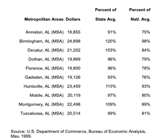
The state’s ten metropolitan areas (MSAs) accounted for 69.3 percent of total sales in 1998, above their 66.6 percent population share. Metro areas are strong draws for shoppers making automotive purchases, with 73.6 percent of automotive sales. They are also a destination for dining out, accounting for 70 percent of sales of eating and drinking places.

Anniston. Sales in the Anniston metropolitan area grew at a state-average 6.0 percent in 1998, second highest among the MSAs, to total $978.5 million. Hardware and lumber sales were up a sizeable 13.7 percent, while automotive sales climbed 10.6 percent and sales of general merchandise rose 10.5 percent. Furniture sales were 8.4 percent above 1997. However, apparel sales declined 3.4 percent. Sales in Anniston averaged $8,362 per resident in 1998, below the statewide average and ranking seventh. Retail sales in the first four months of 1999 posted a gain of 5.0 percent, highest among the ten MSAs.

Birmingham. The Birmingham MSA saw sales of $8.94 billion in 1998, 23.6 percent of all retail sales statewide. While sales rose $276.4 million over 1997, the gain was a modest 3.2 percent. Sales gains were below the statewide average in every sector. Automotive sales showed the strongest increase, at 6.4 percent. Hardware and lumber sales rose 5.3 percent, while apparel sales were up 4.3 percent and sales at eating and drinking places increased 3.3 percent. Furniture sales were down 4.4 percent from 1997. Still, the Birmingham MSA is a destination for shoppers who reside outside the area. Per capita retail sales of $9,837 ranked second in 1998. Birmingham area sales for the first four months of 1999 were flat.

Decatur. Propelled by strong growth in sales of hardware and lumber, retail sales in the Decatur MSA climbed 4.7 percent to $1.07 billion in 1998, an increase of $47.9 million over 1997. Hardware and lumber sales were up 20.4 percent, while automotive sales increased 8.2 percent and sales of general merchandise rose 5.4 percent. However, sales of apparel and furniture, as well as sales at eating and drinking places, fell moderately. The retail draw of the Decatur area continues to be weak, with residents likely to shop for some items outside the area. At $7,481, sales per resident ranked last among the MSAs. Sales rose 3.0 percent during the first four months of 1999 compared to the same period in 1998.

Dothan. Dothan’s retail sector has shown rapid growth in the last two years. From 1996 to 1997, sales jumped 13.2 percent. Area sales rose 7.2 percent from 1997 to 1998, the largest increase among the MSAs. Sales totaled $1.45 billion in 1998, with per capita sales amounting to $10,767, highest among the ten metro areas. This indicates substantial in-shopping by residents from nearby counties in Alabama, Georgia, and Florida. Sales of hardware and lumber climbed 14.7 percent for the year, while automotive sales increased 11.8 percent and general merchandise sales grew 8.8 percent. Although apparel sales were flat, the remaining sectors saw moderate increases. However, for the first four months of 1999, sales gains were a weak 1.0 percent.

Florence. The Florence MSA saw a 2.8 percent gain in retail sales in 1998. This increase of $35.9 million brought the total to $1.32 billion for the year. Growth was below the state average across all sectors. Strongest gains were in general merchandise sales, up 8.8 percent, and sales of hardware and lumber, which rose 7.4 percent. Automotive sales gained just 3.6 percent, compared to Alabama’s statewide increase of 7.8 percent. Sales of furniture and at eating places were flat, while apparel sales declined. Yet, with its location in the northwest corner of the state, the Florence area is a draw for shoppers. Per capita retail sales of $9,600 were almost $900 above the Alabama average and ranked third among the MSAs. Retail sales for the first four months of 1999 rose 2.9 percent.

Gadsden. Gadsden continues to lose a share of its residents’ retail dollars to neighboring areas, including the Birmingham MSA. Retail sales per resident averaged $7,621 in 1998, over $1,000 below the state average, giving the area a ninth place ranking. Retail sales rose $28.4 million during 1998, for a 3.7 percent gain that brought the total to $792.4 million. Hardware and lumber sales showed a strong 11.3 percent gain, while sales at general merchandise stores climbed 7.6 percent. Automotive sales posted a 5.9 percent increase during 1998 and sales at eating places rose 5.7 percent. While apparel sales were up 3.7 percent, furniture sales declined. Sales gains for the first four months of 1999 amounted to 3.2 percent.

Huntsville. Retail sales increased just 1.3 percent in the Huntsville MSA during 1998, the slowest growth of the ten metropolitan areas. Sales totaled $2.7 billion, $35.9 million above the 1997 total. Hardware and lumber rang up the largest gain, at 8.0 percent. Automotive sales were up just 3.4 percent. A 2.0 percent increase in sales at general merchandise stores compares to the 10.1 percent average gain statewide. Sales at eating places were flat, while apparel and furniture sales declined. Huntsville ranked eighth on per capita sales, with an average of $7,941 in retail purchases per resident. The first four months of 1999 saw a stronger sales increase of 2.3 percent.

Mobile. Mobile area retail sales were dampened by the effects of Hurricane Georges in the fall of 1998, with the gain for the year just 2.2 percent. This $98.0 million increase brought area retail sales to $4.55 billion for 1998. Per capita sales of $8,544 were slightly below the Alabama average and ranked the area sixth. The largest gains in 1998 came from automotive sales, which were 8.3 percent above the 1997 total. Sales at eating places showed the strongest growth among the ten MSAs, increasing 6.3 percent. Hardware and lumber sales rose 5.7 percent. Furniture sales were up slightly, but sales of general mer- chandise and apparel declined. Retail growth continued at a 2.3 percent pace through April 1999.

Montgomery. The Montgomery MSA posted a below-average 2.5 percent increase in retail sales during 1998. Sales for the year totaled $2.97 billion, an increase of $73.1 million. Auto- motive sales gains of 8.2 percent bested the state average of 7.8 percent. However, hardware and lumber sales increased just 3.1 percent, while sales of general merchandise were off 2.9 percent from 1997. There were modest increases in furniture and apparel sales and in sales at eating places. Montgomery area sales averaged $9,237 per resident, over $500 above the state average, to rank fifth. Sales for the first four months of 1999 rose 2.3 percent.

Tuscaloosa. An increase in retail sales of 5.8 percent ranked Tuscaloosa third among the MSAs in sales growth during 1998. Sales for the year totaled $1.51 billion, up $82.9 million from 1997. Strong automotive sales were largely responsible for the increase. Automotive sales jumped 15.4 percent in 1998, compared to a statewide average sales increase of 7.8 percent. Sales at eating and drinking places were also strong, posting a 6.2 percent gain. General merchandise sales rose 5.3 percent, while sales of apparel were up 4.6 percent. Hardware and lumber and furniture posted weak increases of just over one percent. Per capita retail sales of $9,404 were about $700 above the state average and ranked fourth. Through April 1999, sales growth has been a moderate 2.3 percent.

Carolyn Trent

Retail Sales in Alabama MSAs, 1994-1998
($1,000)

						Percent
						Change
Area	1994	1995	1996	1997	1998	1997-1998
Alabama	31,007,474	32,887,390	34,541,611	35,748,153	37,900,661	6.0
Anniston	801,800	840,939	867,420	923,369	978,487	6.0
Birmingham	7,776,310	8,175,265	8,403,847	8,660,976	8,937,370	3.2
Decatur	906,328	946,314	970,562	1,020,546	1,068,451	4.7
Dothan	1,095,653	1,170,757	1,195,669	1,353,706	1,450,895	7.2
Florence	1,096,925	1,137,270	1,176,661	1,281,963	1,317,841	2.8
Gadsden	637,358	669,411	693,011	763,951	792,351	3.7
Huntsville	2,361,918	2,420,503	2,499,907	2,667,462	2,703,347	1.3
Mobile	3,753,898	3,967,801	4,142,801	4,449,458	4,547,443	2.2
Montgomery	2,633,212	2,708,439	2,819,778	2,899,193	2,972,300	2.5
Tuscaloosa	1,194,335	1,255,795	1,292,325	1,428,993	1,511,893	5.8

Source: Center for Business and Economic Research, The University of Alabama.

Public Education: A Crisis in Confidence?

July 26th, 2019

Public Education: A Crisis in Confidence?

In 1970, Alabama per capita income was $2,964 compared to $4,077 for the United States. Per capita income in Alabama was 73 percent of the national average. By 1998, this gap had shrunk—Alabama income was 81 percent of the national average. Alabama 1998 per capita income was estimated to be $21,442 compared to $26,412 for the United States.

While the income gap between Alabama and the national average has narrowed over the past 30 years, why Alabama persistently lags behind our sister states demands understanding. Why does the average Alabamian earn less than the average American? There are two primary reasons. First, many rural Alabama counties have little or no industry. These counties have high unemployment and significant poverty. Tables 1 and 2 give data for all 67 counties and profile Alabama’s 10 poorest and 10 wealthiest counties.

The second reason for the income gap is in the nature of the industries that dominate Alabama’s rural industrial base. The common thread among rural Alabama employers is their minimal labor force requirements. Rural Alabama employment is dominated by low skill, low wage industries—characteristic of a poorly educated workforce.

Alabama is a state blessed with natural resources. It is located in one of the fastest growing regions

of the country, and it connects to superb domestic and international markets by air, rail, interstate, and sea. Why then does the state continue to under-perform the nation as a whole?

As in all matters of the human condition, there are many forces at work. Alabama lives with a legacy that extends to the Civil War and before. While the land and climate are well suited to an agrarian economy, an agrarian economy is not the wealth producer in the 20th century that it was in the 18th. Rural Alabama is struggling to find its place in an increasingly information and technology driven economy—a 21st century economy that demands a well-educated workforce.

In 1970, 25.9 percent of the Alabama population had at least a high school education compared to 31.1 percent for the United States. Educational attainment in the state has risen in the past 30 years, but has not caught up to the national average. Herein lies a clue to Alabama’s income disparity. In 1998, 78.8 percent of adult Alabamians had at least a high school education compared to 82.8 percent for the United States. State wide numbers don’t tell the whole story. The average educational attainment of the adults in the urban counties is significantly higher than that of the adults in the rural counties. Our urban centers, home of the state’s good public schools and most of the colleges and universities, are also home of Alabama’s 21st century employment opportunities.

These observations are a bit like a child’s marveling at the discovery that the sun always rises in the east. How can one deny that the quality of life and the future of the economy are contingent on a well-educated citizenry? This issue is rarely de- bated. So why then does Alabama seem to ignore the quality of education in the rural counties? And why, at times of need in urban schools, are public tax referendums frequently defeated?

As new communities sprang up in the westward movement across America, settlers first built shelter, then a church, and then a school. Young families and grandparents alike knew the value of education. They built the school with their own hands and hired the teacher. They understood the value of an education and they invested their time and personal wealth in the future of the children of the community. They saw these expenditures as an investment. They knew that one day the children would become teachers, doctors, business leaders, architects of tomorrow— builders of the future.

Maybe Alabama faces crisis of confidence. Confidence in the ability of the schools to teach and educate the children, the confidence once born of involvement, has been lost through the pace and distractions of late 20th century living.

For Alabama to prosper, to begin to realize its economic potential, it must be willing to invest in all of its children. This will only happen when every adult once again believes in the value of education and the ability of our schools to teach and educate the children of Alabama—the leaders and workers of tomorrow.

State Poverty Estimates for 1996 Released

July 26th, 2019

State Poverty Estimates for 1996 Released

Estimates recently released by the Census Bureau put the number of Alabamians in poverty in 1996 at 733,113, or 17.1 percent of the state’s total population. This number is down from an estimated 752,097 residents (17.6 percent of the total) in poverty in 1995. Alabama’s 2.5 percent decrease contrasts with a 0.3 percent increase in the total number of poor Americans. However, Alabama continues to rank 42nd among the 50 states on the percentage of all residents in poverty.

Poverty rates in 1996 were still much worse for children throughout the U.S. Almost 30 (29.6) percent of Alabama preschoolers live in poverty. Nationwide, the percentage is about 23.4. School-aged children (ages 5 to 17) also experience higher poverty rates than the general population. In Alabama, an estimated 22.9 percent of related children aged 5 to 17 lived in poor families in 1996. Across the U.S., the estimate was 18.6 percent.

The Census Bureau’s 1996 estimates are based on the March 1997 Current Population Survey as well as records on food stamp recipients, income tax returns, and the 1990 census. While national and state estimates are issued annually, county and school district estimates of poverty are provided semiannually in odd-numbered years.

Category: Research Library

Category: Research Library

Alabama Gains Residents from Migration in 1997-98